Under the hood
Disk Models
Model Handling
You should define the model with the ModelSersic() class :
from galpak import GalPaK3D, ModelSersic
mymodel = ModelSersic(flux_profile='exponential',rotation_curve='tanh',redshift=1.0)
gk = GalPaK3D('GalPaK_cube_1101_from_paper.fits',model=mymodel)
And print(gk.model) should yield
Note
The galpak save() method will save a file model.txt
If the model is saved into a model.txt file, one can use :
from galpak import GalPaK3D
gk = GalPaK3D('GalPaK_cube_1101_from_paper.fits',model='model.txt')
The file model.txt should be like :
Base Model Class
- galpak.DefaultModel
alias of
galpak.model_sersic3d.ModelSersic
- class galpak.ModelSersic(flux_profile='exponential', thickness_profile='gaussian', dispersion_profile='thick', rotation_curve='tanh', flux_image=None, line=None, aspect=None, redshift=None, pixscale=None, cosmology='planck15')[source]
The first and default galpak Model (when unspecified). It simulates a simple disk galaxy using DiskParameters.
- flux_profile: ‘exponential’ | ‘gaussian’ | ‘de_vaucouleurs’ | ‘sersicN2’ | ‘user’
The flux profile of the observed galaxy. The default is ‘exponential’. See http://en.wikipedia.org/wiki/Sersic%27s_law If ‘user’ provided flux map, specify flux_image. Currently unsupported
- thickness_profile: ‘gaussian’ [default] | ‘exponential’ | ‘sech2’ | ‘none’
The perpendicular flux profile of the disk galaxy. The default is ‘gaussian’. If none. the galaxy will become a cylinder.
- rotation_curve: ‘arctan’ | ‘exponential’ | ‘tanh’ [default] |
‘isothermal’ | ‘NFW’ | ‘Burkert’ | ‘mass’ | ‘Freeman’ | ‘Spano’
- The profile of the velocity v(r) can be in (with X=r/rV where rV=turnover radius):
arctan : Vmax arctan(X),
tanh : Vmax tanh(X),
exponential : inverted exponential, Vmax (1-exp(-X))
isothermal : for an isothermal halo, Vmax [1-arctan(X)/X)]^0.5
NFW : for a NFW halo, Vmax {[ln(1+X) - X/(1+X)]/X}^0.5
Burkert : for a Burkert halo, Vmax {[ln(1 + X) + 0.5 ln (1 + X^2) - arctan(X)]/X}^0.5
Freeman : a Freeman disk with Vmax=V2.2
mass : a constant light-to-mass ratio v(r)=sqrt(G m(<r) / r); where m(<r) is the cumulative mass profile with m(<r) = int I(r) 2 pi r dr
- Spano: for a Spano 2008 profile, Vmax {arcsinh(X)/X - 1/sqrt(1+X2)}
The default is ‘tanh’.
- dispersion_profile: ‘thick’ [default] | ‘thin’
The local disk dispersion from the rotation curve and disk thickness from Binney & Tremaine 2008, see Genzel et al. 2008. GalPak has 3 components for the dispersion:
a component from the rotation curve arising from mixing velocities of a disk with non-zero thickness.
a component from the local disk dispersion specified by disk_dispersion
a spatially constant dispersion, which is the output parameter velocity_dispersion.
- line: None[default] | dict to fit doublets, use a dictionary with
line[‘wave’]=[l, lref] eg. [3726.2, 3728.9] # Observed or Rest
line[‘ratio’]=[0.8, 1.0] eg. [0.8, 1.0] # The primary line for redshifts is the reddest
- redshift: float
The redshift of the observed galaxy, used in mass calculus. Will override the redshift provided at init ; this is a convenience parameter. If this is not set anywhere, GalPak will not try to compute the mass.
- galpak.DiskModel
alias of
galpak.model_sersic3d.ModelSersic
Instruments
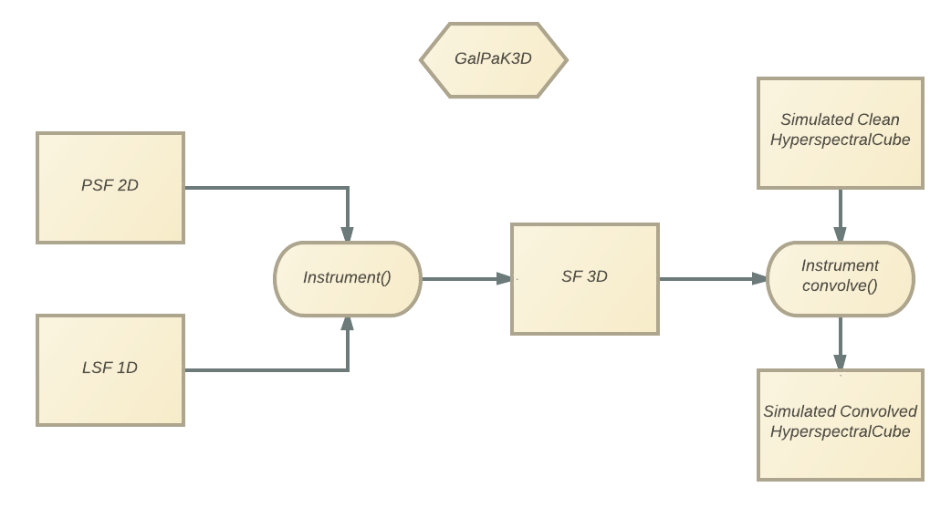
GalPaK uses a virtual Instrument
to convolve the simulation cubes and check against observed data.
As each instrument has its own tweaks and quirks (both hardware and atmospheric),
you can provide an instrument to GalPaK3D,
the default one being MUSE in Wide Field Mode :
The spectral characteristics (pixel cdelt, etc.) are re-calibrated using the Cube’s header when you instantiate GalPaK.
Pay attention in defining most appropriate values for the seeing or psf_fwhm(“)
– psf_ba if not round – and lsf_fwhm (in units of cube) parameters.
All of them by default use the gaussian PSF GaussianPointSpreadFunction.
Instruments handling
You should define the instrument as :
from galpak import GalPaK3D, MUSE, GaussianPointSpreadFunction
mypsf = GaussianPointSpreadFunction(fwhm=0.7,pa=0,ba=1)
myinstr = MUSE(psf=mypsf,lsf=None)
gk = GalPaK3D('GalPaK_cube_1101_from_paper.fits',instrument=myinstr)
And print(gk.instrument) should yield
Note
The galpak save method will save a file instrument.txt
If the instrument is saved into a instrument.txt file, one can use :
from galpak import GalPaK3D
gk = GalPaK3D('GalPaK_cube_1101_from_paper.fits',instrument='instrument.txt')
The file instrument.txt should be like :
Note
Both instrument.txt and model.txt can be combined in a single config file
Instruments supported
- ALMA
set lsf_fwhm to 1 cdelt (default) or less or use NoLineSpreadFunction
- SINFONI (J250, H250 and K250 modes)
SINFOJ250, SINFOH250, SINFOK250 :
- from galpak import run, SINFOK250
gk = run(‘my_sinfok250_cube.fits’, instrument=SINFOK250())
- MUSE (WFM and NFW modes)
default lsf_fwhm is 2.67 Angstrom
- KMOS
default xy_step is 0.2 arcsecs
- HARMONI
use the syntax HARMONI(pixscale=30)
OSIRIS
MANGA (soon)
Note
The default Instrument values will be overridden by the cube header info (CRPIX, CDELT etc.) if present.
Base Instrument Class
- class galpak.Instrument(psf=None, lsf=None)[source]
This is a generic instrument class to use or extend.
- psf: None|PointSpreadFunction
The 2D Point Spread Function instance to use in the convolution, or None (the default). When this parameter is None, the instrument’s PSF will not be applied to the cube.
- lsf: None|LineSpreadFunction
The 1D Line Spread Function instance to use in the convolution, or None (the default). Will be used in the convolution to spread the PSF 2D image through a third axis, z. When this parameter is None, the instrument’s PSF will not be applied to the cube.
- convolve(cube)[source]
Convolve the provided data cube using the 3D Spread Function made from the 2D PSF and 1D LSF. Should transform the input cube and return it. If the PSF or LSF is None, it will do nothing.
Warning
The 3D spread function and its fast fourier transform are memoized for optimization, so if you change the instrument’s parameters after a first run, the SF might not reflect your changes. Delete
psf3dandpsf3d_fftto clear the memory.cube: HyperspectralCube
Hyperspectral Cube
This class is a very simple (understand : not fully-featured nor exhaustive) model of a hyperspectral cube.
- class galpak.HyperspectralCube(data=None, header=None, verbose=False, filename=None, variance=None)[source]
A hyperspectral cube has 3 dimensions : 2 spatial, and 1 spectral. It is basically a rectangular region of the sky seen on a discrete subset of the light spectrum. It is heavily used in spectral imaging, and is provided by spectroscopic explorers such as MUSE.
This class is essentially a convenience wrapper for data values and header specs of a single hyperspectral cube.
It understands the basic arithmetic operations
+ - * / **, which should behave much like with numpy’s ndarrays, and update the header accordingly. An operation between a cube and a number will behave as expected, by applying the operation voxel-by-voxel to the cube. (it broadcasts the number to the shape of the cube) An operation between a cube and an image (a slice along the spectral axis, z) will behave as expected, by applying the operation image-by-image to the cube. (it broadcasts the image to the shape of the cube)It also understands indexation of the form
cube[zmin:zmax, ymin:ymax, xmin:xmax].See also http://en.wikipedia.org/wiki/Hyperspectral_imaging .
Note : no FSCALE management is implemented yet.
You can load from a single HDU of a FITS (Flexible Image Transport System) file :
HyperspectralCube.from_file(filename, hdu_index=None, verbose=False)
- data: numpy.ndarray|None
3D numpy ndarray holding the raw data. The indices are the pixel coordinates in the cube. Note that in order to be consistent with astropy.io.fits, data is indexed in that order : λ, y, x.
- header: fits.Header|None
http://docs.astropy.org/en/latest/io/fits/api/headers.html Note: this might become its own wrapper class in the future.
- verbose: boolean
Set to True to log everything and anything.
- defaults_from_instrument(instrument=None)[source]
- First reads the header for
xy_step (CDELT1 or CD1_1) z_step (CDELT3 or CD3_3) z_cunit (CUNIT3) crpix (CRPIX3) crval (CRVAL3).
If some of these are None, get the default values from the instrument and then reset the header :
xy_step: Instrument.xy_step –> self.xy_step z_step: Instrument.z_step –> self.z_step –> CDELT3 z_cunit: Instrument.z_cunit –> self.z_cunit –> CUNIT3 crpix: shape[0]/2 –> CRPIX3 crval: Instrument.z_central –> self.z_central –> CRVAL3
for CUNIT3 CRVAL3 CRPIX3 CDELT3
- static from_file(filename, hdu_index=None, verbose=False)[source]
Factory to create a HyperspectralCube from one HDU in a FITS file. http://fits.gsfc.nasa.gov/fits_standard.html
No other file formats are supported at the moment. You may specify the index of the HDU you want. If you don’t, it will try to guess by searching for a HDU with EXTNAME=DATA, or it will pick the first HDU in the list that has 3 dimensions.
- filename: string
An absolute or relative path to the FITS file we want to load. The astropy.io.fits module is used to open the file.
- hdu_index: integer|None
Index of the HDU to load. If you set this, guessing is not attempted.
- verbose: boolean
Should we fill up the log with endless chatter ?
- Return type
- get_steps()[source]
Returns a list of the 3 steps [λ,y,x]. The units are the ones specified in the header.
- initialize_self_cube()[source]
Initialize steps xy_steps z_steps z_cunnit and z_central z_central requires CRPIX3 CRVAL3 CDELT3
- initialize_self_cube()[source]
Initialize steps xy_steps z_steps z_cunnit and z_central z_central requires CRPIX3 CRVAL3 CDELT3
- sanitize(header=None, data=None)[source]
Procedurally apply various sanitization tasks : - http://docs.astropy.org/en/latest/io/fits/usage/verification.html (todo) - Fix spectral step keyword :
CDEL_3 –> CDELT3
CD3_3 –> CDELT3
- Fix blatantly illegal units :
DEG –> deg
MICRONS –> um
Sanitizes this cube’s header and data, or provided header and data.
Warning
header and data are mutated, not copied, so this method returns nothing.
Note
This class is not fully formed yet and its API may evolve as it moves to its own module.
Important
A description of the parameter meaning can be found here
- class galpak.GalaxyParameters(x=None, y=None, z=None, flux=None, radius=None, inclination=None, pa=None, turnover_radius=None, maximum_velocity=None, velocity_dispersion=None)[source]
A simple wrapper for an array of galaxy parameters. It is basically a flat numpy.ndarray of a bunch of floats with convenience attributes for explicit (and autocompleted!) access and mutation of parameters, and nice casting to string.
Warning
Undefined parameters will be NaN, not None.
Example :
from galpak import GalaxyParameters
gp = GalaxyParameters(x=1.618)

// Classic numpy.ndarray numeric access
assert(gp[0] == 1.618)
// Autocompleted and documented property access
assert(gp.x == 1.618)
// Convenience dictionary access,
assert(gp['x'] == 1.618)
// ... useful when you're iterating :
for (name in GalaxyParameters.names):
    print gp[name]
- Parameters :
x (pix)
y (pix)
z (pix)
flux
- radius aka. r½ (pix)
half-light radius in pixel
inclination (deg)
- pa (deg)
position angle from y-axis, anti-clockwise.
- turnover_radius aka. rv (pix)
turnover radius for arctan, exp, velocity profile [is ignored for mass profile]
- maximum_velocity aka. Vmax (km/s)
de-projected V_max [forced to be positive, with 180deg added to PA]
velocity_dispersion aka. s0 (km/s)
Note that all the parameters are lowercase, even if they’re sometimes displayed mixed-case.
- Additional attributes :
- stdevOptional stdev margin (GalaxyParametersError).
GalPaK3D fills up this attribute.
- static from_ndarray(a)[source]
Factory to easily create a GalaxyParameters object from an ordered ndarray whose elements are in the order of GalaxyParameters.names.
Use like this :
from galpak import GalaxyParameters
gp = GalaxyParameters.from_ndarray(my_ndarray_of_data)
- Return type
Description
A GalaxyParameters object gp is merely a glorified numpy.ndarray with convenience accessors and mutators :
Warning
the velocity_dispersion parameter is NOT the total dispersion. This parameter is akin to a turbulent term. It is added in quadrature to the dispersions due to the disk model and to the thickness. See Cresci et al. 2009, Genzel et al. 2011, and Bouche et al. 2015
You still can access the parameters like an indexed array
assert gp.x == gp[0]  # true
assert gp.y == gp[1]  # true
# ...
assert gp.sigma0 == gp[9]  # true
You may instantiate a GalaxyParameters object like so
from galpak import GalaxyParameters

gp = GalaxyParameters(z=0.65)
gp.x = 5.
assert gp.z == 0.65       # true
assert gp.x == 5.         # true
Warning
An undefined value in GalaxyParameters will be nan, not None
assert math.isnan(gp.pa)  # true
assert gp.pa is None      # false
Getting the Wavelength
The z attribute in a GalaxyParameter is in pixels,
you may want the value in the physical unit specified in your Cube’s header.
To that effect, you may use the wavelength_of method of the HyperspectralCube:
from galpak import GalPaK3D
gk = GalPaK3D('my_muse_cube.fits')
gk.run_mcmc()

wavelength = gk.cube.wavelength_of(gk.galaxy.z)
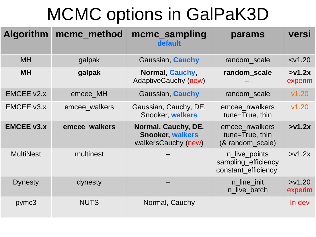
MCMC
GalPaK3D allows the user to select several samplers for the MCMC as described in the
run_mcmc method which has the following options:
- mcmc_method: ‘galpak’ [default] | ‘emcee_walkers’| ‘emcee_MH’ | ‘dynesty’ | ‘multinest’
- The MCMC method.
galpak: for the original MCMC algorithm using Cauchy proposal distribution
emcee_MH: emcee v2.x classic MH; no longer supported
emcee_walkers: emcee v3.x multi-Walkers algorithms with Moves
dynesty: unsupported
multinest: still experimental
pymc3: to be implemented
- mcmc_sampling:
galpak: ‘Cauchy’ [default] | ‘Normal’ | ‘AdaptiveCauchy’
emcee_walkers: ‘walkers’ [default] | ‘walkersCauchy’ | ‘DE’ | ‘Snooker’ | ‘Cauchy’ | ‘Normal’
multinest: None
pymc3: to be implemented
The proposal sampling methods
GalPaK3D uses an internal MCMC class which extend the galpak class.
This can be used to call its likelihood such as:
li = gk(params)
using a self.__call__() method which returns the lnprob
Here is a full example:
import galpak
gk=galpak.GalPaK3D('data/input/GalPaK_cube_1101_from_paper.fits',model=galpak.DefaultModel())
p=gk.model.Parameters()
params=p.from_ndarray([15,15,15,1e-16,5,60,90,1,100,10])
li=gk(params)
You can always check that the log-likelihood is finite :
print(li)
-16117.55742040931
If it is not finite, this is probably caused by the priors when the parameter values are outside the min and max boundaries.
- class galpak.MCMC[source]
An extension of the galpak class with the galpak MH algorithm (myMCMC class) and method used for emcee and external algorithm
- the following methods are for external samplers such as emcee:
lnprob: returned by __call__ / the full log-probability function: Ln = Priors x L(p)
loglike: the log L(p)
logpriors: the log priors with uniform priors.
- the following methods are for multinest:
pyloglike: the log L(p)
pycube: transforms unit cube to uniform priors.
- the following methods are for dynesty:
loglike: the log L(p)
ptforms: transforms unit cube to uniform priors.
- the following methods are for the internal galpak MH algorithm
myMCMC
Point Spread Functions
GalPaK provides the two most common PSF : Gaussian and Moffat.
You may use them as the psf argument of the Instrument, as described here.
All instruments use this PSF model by default, with their own configuration :
- class galpak.GaussianPointSpreadFunction(fwhm=None, pa=0, ba=1.0)[source]
The default Gaussian Point Spread Function.
- fwhm: float
Full Width Half Maximum in arcsec, aka. “seeing”.
- pa: float [default is 0.]
Position Angle of major-axis, anti-clockwise rotation from Y-axis, in angular degrees.
- ba: float [default is 1.0]
Axis ratio of the ellipsis, b/a ratio (y/x).
- class galpak.MoffatPointSpreadFunction(fwhm=None, alpha=None, beta=None, pa=0, ba=1)[source]
The Moffat Point Spread Function
- fwhm if alpha is None: float [in arcsec]
Moffat’s distribution fwhm variable : http://en.wikipedia.org/wiki/Moffat_distribution
- alpha if fwhm is None: float [in arcsec]
Moffat’s distribution alpha variable : http://en.wikipedia.org/wiki/Moffat_distribution
- beta: float
Moffat’s distribution beta variable : http://en.wikipedia.org/wiki/Moffat_distribution
- pa: float [default is 0.]
Position Angle of major-axis, the anti-clockwise rotation from Y, in angular degrees.
- ba: float [default is 1.0]
Axis ratio of the ellipsis, b/a ratio (y/x).
In order to furthermore customize the PSF you want to use, you can create your own PSF class and use it in the instrument, it simply needs to implement the following interface :
Line Spread Functions
GalPaK provides two LSFs : Gaussian and MUSE. These are used to extrude the 2D PSF image into 3D, right before its application in Fourier space.
You may use them as the lsf argument of the Instrument,
as described here.
All instruments use this LSF model by default, with their own configuration :
- class galpak.GaussianLineSpreadFunction(fwhm)[source]
A line spread function that spreads as a gaussian. We assume the centroid is in the middle.
- fwhm: float
Full Width Half Maximum, in units of CUNIT3
This LSF requires the mpdaf module, specifically mpdaf.MUSE.LSF.
As this LSF is optional, you must explicitly tell your instrument to use it when you want to.
- class galpak.MUSELineSpreadFunction(model='qsim_v1')[source]
A line spread function that uses MPDAF’s LSF. See http://urania1.univ-lyon1.fr/mpdaf/chrome/site/DocCoreLib/user_manual_PSF.html
Warning
This requires the mpdaf module. Currently, the MPDAF module only works for odd arrays.
- model: string
See
mpdaf.MUSE.LSF’stypparameter.
In order to further customize the LSF you want to use, you can create your own LSF class and use it in the instrument, it simply needs to implement the following interface :