A quick overview
The algorithm directly compares data-cubes with a disk parametric model which has 9 or 10 free parameters [which can also be fixed independently]. The algorithm uses a Markov Chain Monte Carlo (MCMC) approach with non-traditional sampling laws in order to efficiently probe the parameter space. More importantly, it uses the knowledge of the 3-dimensional spread-function to return the intrinsic galaxy properties and the intrinsic data-cube. The 3D spread-function class is flexible enough to handle any instrument.
One can use such an algorithm to constrain simultaneously the kinematics and morphological parameters of (non-merging, i.e. regular) galaxies observed in non optimal seeing conditions. The algorithm can also be used on Adaptive-Optics (AO) data or on high-quality, high-SNR data to look for non-axisymmetric structures in the residuals.
The algorithm can be (roughly) summarized as :
Pick new random galaxy parameters using uniform priors [boundaries can be set]
Create clean cube from parameters and convolve it with instrument’s PSF+LSF
Measure closeness of resulting convolved cube to input cube
Accept/Reject galaxy parameters using Metropolis-Hasting algorithm
Goto 1. until max iterations are reached
Fill output attributes with data (chain, cubes, etc.)
Compute and return best fit galaxy parameters from chain
Warning
The output flux is in the pixel units, which may need to multiplied by CDELT3.
Warning
- The algorithm should never be used blindly and we stress that one should always
look at the convergence of the parameters using
plot_mcmc(),investigate possible covariance in the parameters using
plot_correlations()and/or fix a parameter with the option known_parameters to remove the degenerancy,adjust the MCMC algorithm with the option random_scale (lower than 1 [default] for higher acceptance rate and vice versa) to ensure an acceptance rate of 30 to 50%.
Parameter meaning
Important
A description of the parameter meaning can be found here
- class galpak.GalaxyParameters(x=None, y=None, z=None, flux=None, radius=None, inclination=None, pa=None, turnover_radius=None, maximum_velocity=None, velocity_dispersion=None)[source]
A simple wrapper for an array of galaxy parameters. It is basically a flat numpy.ndarray of a bunch of floats with convenience attributes for explicit (and autocompleted!) access and mutation of parameters, and nice casting to string.
Warning
Undefined parameters will be NaN, not None.
Example :
from galpak import GalaxyParameters
gp = GalaxyParameters(x=1.618)

// Classic numpy.ndarray numeric access
assert(gp[0] == 1.618)
// Autocompleted and documented property access
assert(gp.x == 1.618)
// Convenience dictionary access,
assert(gp['x'] == 1.618)
// ... useful when you're iterating :
for (name in GalaxyParameters.names):
    print gp[name]
- Parameters :
x (pix)
y (pix)
z (pix)
flux
- radius aka. r½ (pix)
half-light radius in pixel
inclination (deg)
- pa (deg)
position angle from y-axis, anti-clockwise.
- turnover_radius aka. rv (pix)
turnover radius for arctan, exp, velocity profile [is ignored for mass profile]
- maximum_velocity aka. Vmax (km/s)
de-projected V_max [forced to be positive, with 180deg added to PA]
velocity_dispersion aka. s0 (km/s)
Note that all the parameters are lowercase, even if they’re sometimes displayed mixed-case.
- Additional attributes :
- stdevOptional stdev margin (GalaxyParametersError).
GalPaK3D fills up this attribute.
- static from_ndarray(a)[source]
Factory to easily create a GalaxyParameters object from an ordered ndarray whose elements are in the order of GalaxyParameters.names.
Use like this :
from galpak import GalaxyParameters
gp = GalaxyParameters.from_ndarray(my_ndarray_of_data)
- Return type
Description
A GalaxyParameters object gp is merely a glorified numpy.ndarray with convenience accessors and mutators :
Warning
the velocity_dispersion parameter is NOT the total dispersion. This parameter is akin to a turbulent term. It is added in quadrature to the dispersions due to the disk model and to the thickness. See Cresci et al. 2009, Genzel et al. 2011, and Bouche et al. 2015
You still can access the parameters like an indexed array
assert gp.x == gp[0]  # true
assert gp.y == gp[1]  # true
# ...
assert gp.sigma0 == gp[9]  # true
You may instantiate a GalaxyParameters object like so
from galpak import GalaxyParameters

gp = GalaxyParameters(z=0.65)
gp.x = 5.
assert gp.z == 0.65       # true
assert gp.x == 5.         # true
Warning
An undefined value in GalaxyParameters will be nan, not None
assert math.isnan(gp.pa)  # true
assert gp.pa is None      # false
Getting the Wavelength
The z attribute in a GalaxyParameter is in pixels,
you may want the value in the physical unit specified in your Cube’s header.
To that effect, you may use the wavelength_of method of the HyperspectralCube:
from galpak import GalPaK3D
gk = GalPaK3D('my_muse_cube.fits')
gk.run_mcmc()

wavelength = gk.cube.wavelength_of(gk.galaxy.z)
Input Cubes supported
Any fits cube can be used provided that the z-axis represents wavelengths or frequencies.
Any units are normally accepted as the algorithm works in velocity space (dlamba/lamba or dfrequency/frequency). Check the Instrument.z_step_kms value which is critial for the kinematic parameters.
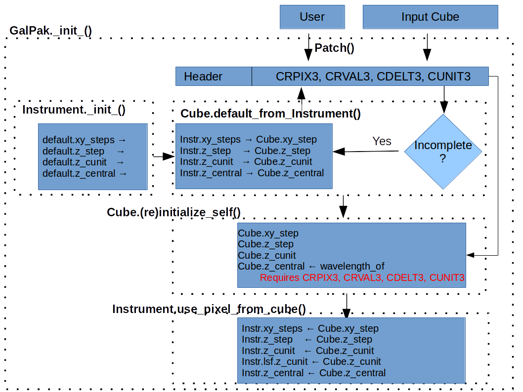
If the header is incomplete (CRPIX3, CDELT3, CRVAL3, CUNIT3), the algorithm will try to use the default values assigned to the instrument. The user can specify these directly.
If the header is complete, the instrument default pixel sizes will be over-written by the the information from the cube header.
A MPDAF
Obj.Cubeobject is ok as input.To provide the variance, use a separate file with `variance’ or via a MPDAF Obj.Cube. If no Variance is specified, the (edge of the) cube statistics will be used.
In future versions, the variance can also be specified as a “STAT” or “VARIANCE” extension to the fits file
Warning
Pay attention to the LSF FWHM, which should be specified in the same units as the cube.
Incomplete Header handling overview