Instruments

GalPaK uses a virtual Instrument to convolve the simulation cubes and check against observed data. As each instrument has its own tweaks and quirks (both hardware and atmospheric), you can provide an instrument to GalPaK3D, the default one being MUSE in Wide Field Mode :

The spectral characteristics (pixel cdelt, etc.) are re-calibrated using the Cube’s header when you instantiate GalPaK. Pay attention in defining most appropriate values for the seeing or psf_fwhm(“) – psf_ba if not round – and lsf_fwhm (in units of cube) parameters. All of them by default use the gaussian PSF GaussianPointSpreadFunction.

Instruments handling

You should define the instrument as :

from galpak import GalPaK3D, MUSE, GaussianPointSpreadFunction
mypsf = GaussianPointSpreadFunction(fwhm=0.7,pa=0,ba=1)
myinstr = MUSE(psf=mypsf,lsf=None)
gk = GalPaK3D('GalPaK_cube_1101_from_paper.fits',instrument=myinstr)

And print(gk.instrument) should yield

[INSTRUMENT] :

type = MUSE

pixscale = 0.2 “

[PSF] :

type = gaussian

fwhm = 0.7 “

pa = 0 °

ba = 1

[LSF] :

type = Gaussian

fwhm = 2.5369617016 Angstrom

cube_xy_step = 0.2 “

cube_z_step = 1.25 Angstrom

cube z_step_kms = 57.12979890310786 km/s at 6564.0 Angstrom

Note

The galpak save method will save a file instrument.txt

If the instrument is saved into a instrument.txt file, one can use :

from galpak import GalPaK3D
gk = GalPaK3D('GalPaK_cube_1101_from_paper.fits',instrument='instrument.txt')

The file instrument.txt should be like :

[INSTRUMENT] :

type = MUSE

pixscale = 0.2 “

[PSF] :

type = gaussian

fwhm = 0.7 “

pa = 0 °

ba = 1

[LSF] :

type = Gaussian

fwhm = 2.5369617016 Angstrom

Note

Both instrument.txt and model.txt can be combined in a single config file

Instruments supported

• ALMA

  set lsf_fwhm to 1 cdelt (default) or less or use NoLineSpreadFunction

• SINFONI (J250, H250 and K250 modes)

  SINFOJ250, SINFOH250, SINFOK250 :

  from galpak import run, SINFOK250

  gk = run(‘my_sinfok250_cube.fits’, instrument=SINFOK250())

• MUSE (WFM and NFW modes)

  default lsf_fwhm is 2.67 Angstrom

• KMOS

  default xy_step is 0.2 arcsecs

• HARMONI

  use the syntax HARMONI(pixscale=30)

• OSIRIS

• MANGA (soon)

Note

The default Instrument values will be overridden by the cube header info (CRPIX, CDELT etc.) if present.

Base Instrument Class

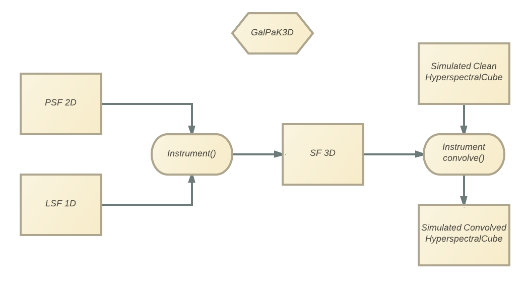
class galpak.Instrument(psf=None, lsf=None)

This is a generic instrument class to use or extend.

psf: None|PointSpreadFunction

The 2D Point Spread Function instance to use in the convolution, or None (the default). When this parameter is None, the instrument’s PSF will not be applied to the cube.

lsf: None|LineSpreadFunction

The 1D Line Spread Function instance to use in the convolution, or None (the default). Will be used in the convolution to spread the PSF 2D image through a third axis, z. When this parameter is None, the instrument’s PSF will not be applied to the cube.

convolve(cube)

Convolve the provided data cube using the 3D Spread Function made from the 2D PSF and 1D LSF. Should transform the input cube and return it. If the PSF or LSF is None, it will do nothing.

Warning

The 3D spread function and its fast fourier transform are memoized for optimization, so if you change the instrument’s parameters after a first run, the SF might not reflect your changes. Delete psf3d and psf3d_fft to clear the memory.

cube: HyperspectralCube